Diagnostic plotting functionality for MCMC redistricting.
Source:R/plot_diagnostics.R
redist.diagplot.Rdredist.diagplot generates several common MCMC diagnostic plots.
redist.diagplot(sumstat,
plot = c("trace", "autocorr", "densplot", "mean", "gelmanrubin"),
logit = FALSE, savename = NULL)
Arguments
- sumstat
A vector, list,
mcmcormcmc.listobject containing a summary statistic of choice.- plot
The type of diagnostic plot to generate: one of "trace", "autocorr", "densplot", "mean", "gelmanrubin". If
plot = "gelmanrubin", the inputsumstatmust be of classmcmc.listorlist.- logit
Flag for whether to apply the logistic transformation for the summary statistic. The default is
FALSE.- savename
Filename to save the plot. Default is
NULL.
Value
Returns a plot of file type .pdf.
Details
This function allows users to generate several standard diagnostic plots from the MCMC literature, as implemented by Plummer et. al (2006). Diagnostic plots implemented include trace plots, autocorrelation plots, density plots, running means, and Gelman-Rubin convergence diagnostics (Gelman & Rubin 1992).
References
Fifield, Benjamin, Michael Higgins, Kosuke Imai and Alexander Tarr. (2016) "A New Automated Redistricting Simulator Using Markov Chain Monte Carlo." Working Paper. Available at http://imai.princeton.edu/research/files/redist.pdf.
Gelman, Andrew and Donald Rubin. (1992) "Inference from iterative simulations using multiple sequences (with discussion)." Statistical Science.
Plummer, Martin, Nicky Best, Kate Cowles and Karen Vines. (2006) "CODA: Convergence Diagnosis and Output Analysis for MCMC." R News.
Examples
# \donttest{
data(fl25)
data(fl25_enum)
data(fl25_adj)
## Get an initial partition
init_plan <- fl25_enum$plans[, 5118]
fl25$init_plan <- init_plan
## 25 precinct, three districts - no pop constraint ##
fl_map <- redist_map(fl25, existing_plan = 'init_plan', adj = fl25_adj)
#> Projecting to CRS 3857
alg_253 <- redist_flip(fl_map, nsims = 10000)
#>
#> ── redist_flip() ───────────────────────────────────────────────────────────────
#>
#> ── Automated Redistricting Simulation Using Markov Chain Monte Carlo ──
#> ℹ Preprocessing data.
#> ℹ Starting swMH().
#> ■ 0% | ETA:10s
#> ■■■■ 11% | ETA: 2s | MH Acceptance: 0.76
#> ■■■■■■■ 21% | ETA: 2s | MH Acceptance: 0.78
#> ■■■■■■■■■■■ 32% | ETA: 1s | MH Acceptance: 0.78
#> ■■■■■■■■■■■■■■ 42% | ETA: 1s | MH Acceptance: 0.78
#> ■■■■■■■■■■■■■■■■■ 53% | ETA: 1s | MH Acceptance: 0.78
#> ■■■■■■■■■■■■■■■■■■■■ 64% | ETA: 1s | MH Acceptance: 0.77
#> ■■■■■■■■■■■■■■■■■■■■■■■ 75% | ETA: 0s | MH Acceptance: 0.78
#> ■■■■■■■■■■■■■■■■■■■■■■■■■■■ 85% | ETA: 0s | MH Acceptance: 0.77
#> ■■■■■■■■■■■■■■■■■■■■■■■■■■■■■■ 96% | ETA: 0s | MH Acceptance: 0.78
#> ■■■■■■■■■■■■■■■■■■■■■■■■■■■■■■■ 100% | ETA: 0s | MH Acceptance: 0.77
#>
## Get Republican Dissimilarity Index from simulations
rep_dmi_253 <- redistmetrics::seg_dissim(alg_253, fl25, mccain, pop) |>
redistmetrics::by_plan(ndists = 3)
## Generate diagnostic plots
redist.diagplot(rep_dmi_253, plot = "trace")
 redist.diagplot(rep_dmi_253, plot = "autocorr")
 redist.diagplot(rep_dmi_253, plot = "densplot")
 redist.diagplot(rep_dmi_253, plot = "mean")
 ## Gelman Rubin needs two chains, so we run a second
alg_253_2 <- redist_flip(fl_map, nsims = 10000)
#>
#> ── redist_flip() ───────────────────────────────────────────────────────────────
#>
#> ── Automated Redistricting Simulation Using Markov Chain Monte Carlo ──
#> ℹ Preprocessing data.
#> ℹ Starting swMH().
#> ■ 0% | ETA: 7s
#> ■■ 5% | ETA: 2s
#> ■■■■■■ 15% | ETA: 2s | MH Acceptance: 0.80
#> ■■■■■■■■■ 25% | ETA: 1s | MH Acceptance: 0.80
#> ■■■■■■■■■■ 31% | ETA: 2s | MH Acceptance: 0.81
#> ■■■■■■■■■■■■■■ 42% | ETA: 1s | MH Acceptance: 0.79
#> ■■■■■■■■■■■■■■■■■ 53% | ETA: 1s | MH Acceptance: 0.79
#> ■■■■■■■■■■■■■■■■■■■■ 63% | ETA: 1s | MH Acceptance: 0.79
#> ■■■■■■■■■■■■■■■■■■■■■■■ 74% | ETA: 1s | MH Acceptance: 0.79
#> ■■■■■■■■■■■■■■■■■■■■■■■■■■■ 85% | ETA: 0s | MH Acceptance: 0.79
#> ■■■■■■■■■■■■■■■■■■■■■■■■■■■■■■ 96% | ETA: 0s | MH Acceptance: 0.79
#> ■■■■■■■■■■■■■■■■■■■■■■■■■■■■■■■ 100% | ETA: 0s | MH Acceptance: 0.79
#>
rep_dmi_253_2 <- redistmetrics::seg_dissim(alg_253_2, fl25, mccain, pop) |>
redistmetrics::by_plan(ndists = 3)
## Make a list out of the objects:
rep_dmi_253_list <- list(rep_dmi_253, rep_dmi_253_2)
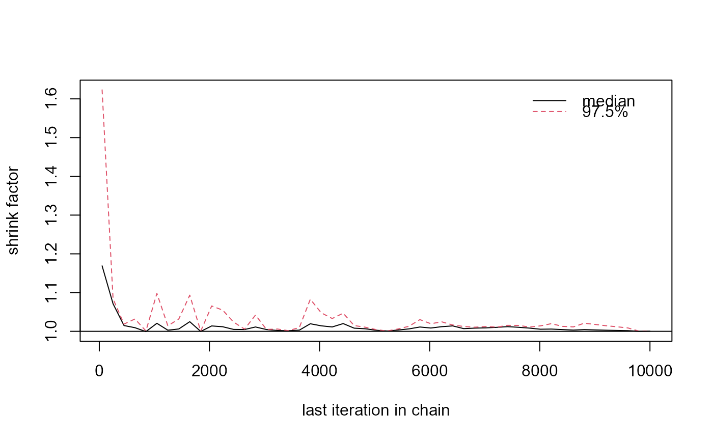
## Generate Gelman Rubin diagnostic plot
redist.diagplot(sumstat = rep_dmi_253_list, plot = "gelmanrubin")
## Gelman Rubin needs two chains, so we run a second
alg_253_2 <- redist_flip(fl_map, nsims = 10000)
#>
#> ── redist_flip() ───────────────────────────────────────────────────────────────
#>
#> ── Automated Redistricting Simulation Using Markov Chain Monte Carlo ──
#> ℹ Preprocessing data.
#> ℹ Starting swMH().
#> ■ 0% | ETA: 7s
#> ■■ 5% | ETA: 2s
#> ■■■■■■ 15% | ETA: 2s | MH Acceptance: 0.80
#> ■■■■■■■■■ 25% | ETA: 1s | MH Acceptance: 0.80
#> ■■■■■■■■■■ 31% | ETA: 2s | MH Acceptance: 0.81
#> ■■■■■■■■■■■■■■ 42% | ETA: 1s | MH Acceptance: 0.79
#> ■■■■■■■■■■■■■■■■■ 53% | ETA: 1s | MH Acceptance: 0.79
#> ■■■■■■■■■■■■■■■■■■■■ 63% | ETA: 1s | MH Acceptance: 0.79
#> ■■■■■■■■■■■■■■■■■■■■■■■ 74% | ETA: 1s | MH Acceptance: 0.79
#> ■■■■■■■■■■■■■■■■■■■■■■■■■■■ 85% | ETA: 0s | MH Acceptance: 0.79
#> ■■■■■■■■■■■■■■■■■■■■■■■■■■■■■■ 96% | ETA: 0s | MH Acceptance: 0.79
#> ■■■■■■■■■■■■■■■■■■■■■■■■■■■■■■■ 100% | ETA: 0s | MH Acceptance: 0.79
#>
rep_dmi_253_2 <- redistmetrics::seg_dissim(alg_253_2, fl25, mccain, pop) |>
redistmetrics::by_plan(ndists = 3)
## Make a list out of the objects:
rep_dmi_253_list <- list(rep_dmi_253, rep_dmi_253_2)
## Generate Gelman Rubin diagnostic plot
redist.diagplot(sumstat = rep_dmi_253_list, plot = "gelmanrubin")
 # }
# }